Welcome to Portal Forecasting!

This is a website run by the Weecology team, comprised of Ethan White’s and Morgan Ernest’s lab groups at the University of Florida. We are a group of interdisciplinary ecologists broadly interested in collaborative approaches to empirical and computation ecology, open science, and open data.

On this website, you’ll find information about our ongoing efforts to forecast a time series of rodent abundances from The Portal project, a long-term experimental monitoring project in desert ecology. Enjoy!

Contributors

Ethan P. White, Glenda M. Yenni, Henry Senyondo, Shawn D. Taylor, Erica M. Christensen, Ellen K. Bledsoe, Juniper L. Simonis, and S. K. Morgan Ernest

Ecological Forecasting

Most forecasts for the future state of ecological systems are conducted once and never updated or assessed. As a result, many available ecological forecasts are not based on the most up-to-date data, and the scientific progress of ecological forecasting models is slowed by a lack of feedback on how well the forecasts perform. Iterative near-term ecological forecasting involves repeated daily to annual scale forecasts of an ecological system and regular assessment of the resulting predictions as new data become available. More frequent updating and assessment will advance ecological forecasting as a field by accelerating the identification of the best models for individual forecasts and improving our understanding of how to best design forecasting approaches for ecology in general.

The Portal Project

The Portal project, located in the Chihuahuan desert of southern Arizona, is a long-term experimental monitoring project in desert ecology. Established in 1977 by Jim Brown, we have over 40 years of data on rodents, plants, ants, and weather at the site. Rodent data are collected approximately monthly, an ideal scenario for short-term forecasts of rodent abundance.

Automated Predictions

The main modeling and forecasting for this project is done using the portalcasting R package (Simonis et al. 2022). We use code in a separate portalPredictions GitHub repository to drive the production forecasts. This code runs automatically once a week on the University’s of Florida’s high performance computing system (the HiPerGator)) and completed forecasts are automatically archived to Zenodo. The translation of the raw Portal Data into model-ready formats is done via the portalr package and the portalcasting package is used to connect the data to the models, execute the models, synthesize the predictions, and produce the output figures.

For further a big picture overview of the system see our paper on this forecasting system (White et al. 2019), but note that due to increased computational demands of the growing model suite and Travis CI’s changes in fee structure, we no longer use Travis CI to run the predictions.

Acknowledgements

This project is developed in active collaboration with DAPPER Stats.

This research was supported in part by the National Science Foundation through grant DEB-1929730 to S.K.M. Ernest and by the Gordon and Betty Moore Foundation’s Data-Driven Discovery Initiative through Grant GBMF4563 to E. P. White.

We thank Hao Ye for feedback on documents and code, Heather Bradley for logistical support, John Abatzoglou for assistance with climate forecasts, and James Brown for establishing the Portal Project.

We currently analyze and forecast rodent data at Portal using fifteen models: AutoARIMA, Seasonal AutoARIMA, ESSS, NaiveARIMA, Seasonal NaiveARIMA, nbGARCH, nbsGARCH, pGARCH, psGARCH, pevGARCH, Random Walk, Logistic, Logistic Covariates, Logistic Competition, Logistic Competition Covariates (WeecologyLab 2019).

AutoARIMA

AutoARIMA (Automatic Auto-Regressive Integrated Moving Average) is a flexible Auto-Regressive Integrated Moving Average (ARIMA) model. ARIMA models are defined according to three model structure parameters – the number of autoregressive terms (p), the degree of differencing (d), and the order of the moving average (q), and are represented as ARIMA(p, d, q) (Box and Jenkins 1970). All submodels are fit and the final model is selected using the auto.arima function in the forecast package (Hyndman and Athanasopoulos 2013; Hyndman 2017). AutoARIMA is fit flexibly, such that the model parameters can vary from fit to fit. Model forecasts are generated using the forecast function from the forecast package (Hyndman and Athanasopoulos 2013; Hyndman 2017). While the auto.arima function allows for seasonal models, the seasonality is hard-coded to be on the same period as the sampling, which is not the case for the Portal rodent surveys. As a result, no seasonal models are evaluated within this model set, but see the sAutoARIMA model. The model is fit using a normal distribution, and as a result can generate negative-valued predictions and forecasts.

Seasonal AutoARIMA

sAutoARIMA (Seasonal Automatic Auto-Regressive Integrated Moving Average) is a flexible Auto-Regressive Integrated Moving Average (ARIMA) model. ARIMA models are defined according to three model structure parameters – the number of autoregressive terms (p), the degree of differencing (d), and the order of the moving average (q), and are represented as ARIMA(p, d, q) (Box and Jenkins 1970). All submodels are fit and the final model is selected using the auto.arima function in the forecast package (Hyndman and Athanasopoulos 2013; Hyndman 2017). sAutoARIMA is fit flexibly, such that the model parameters can vary from fit to fit. Model forecasts are generated using the forecast function from the forecast package (Hyndman and Athanasopoulos 2013; Hyndman 2017). While the auto.arima function allows for seasonal models, the seasonality is hard-coded to be on the same period as the sampling, which is not the case for the Portal rodent surveys. We therefore use two Fourier series terms (sin and cos of the fraction of the year) as external regressors to achieve the seasonal dynamics in the sAutoARIMA model. The model is fit using a normal distribution, and as a result can generate negative-valued predictions and forecasts.

ESSS

ESSS (Exponential Smoothing State Space) is a flexible exponential smoothing state space model (Hyndman et al. 2008). The model is fit using the ets function in the forecast package (Hyndman 2017) with the allow.multiplicative.trend argument set to TRUE. Model forecasts are generated using the forecast function from the forecast package (Hyndman and Athanasopoulos 2013; Hyndman 2017). Models fit using ets implement what is known as the “innovations” approach to state space modeling, which assumes a single source of noise that is equivalent for the process and observation errors (Hyndman et al. 2008). In general, ESSS models are defined according to three model structure parameters – error type, trend type, and seasonality type (Hyndman et al. 2008). Each of the parameters can be an N (none), A (additive), or M (multiplicative) state (Hyndman et al. 2008). However, because of the difference in period between seasonality and sampling of the Portal rodents combined with the hard-coded single period of the ets function, we do not include the seasonal components to the ESSS model. ESSS is fit flexibly, such that the model parameters can vary from fit to fit. The model is fit using a normal distribution, and as a result can generate negative-valued predictions and forecasts.

NaiveARIMA

NaiveARIMA (Naive Auto-Regressive Integrated Moving Average) is a fixed Auto-Regressive Integrated Moving Average (ARIMA) model of order (0,1,0). The model is fit using the Arima function in the forecast package (Hyndman and Athanasopoulos 2013; Hyndman 2017). Model forecasts are generated using the forecast function from the forecast package (Hyndman and Athanasopoulos 2013; Hyndman 2017). While the Arima function allows for seasonal models, the seasonality is hard-coded to be on the same period as the sampling, which is not the case for the Portal rodent surveys. As a result, NaiveARIMA does not include seasonal terms, but see the sNaiveARIMA model. The model is fit using a normal distribution, and as a result can generate negative-valued predictions and forecasts.

Seasonal NaiveARIMA

sNaiveARIMA (Seasonal Naive Auto-Regressive Integrated Moving Average) is a fixed Auto-Regressive Integrated Moving Average (ARIMA) model of order (0,1,0). The model is fit using the Arima function in the forecast package (Hyndman and Athanasopoulos 2013; Hyndman 2017). Model forecasts are generated using the forecast function from the forecast package (Hyndman and Athanasopoulos 2013; Hyndman 2017). While the Arima function allows for seasonal models, the seasonality is hard-coded to be on the same period as the sampling, which is not the case for the Portal rodent surveys. We therefore use two Fourier series terms (sin and cos of the fraction of the year) as external regressors to achieve the seasonal dynamics in the NaiveARIMA model. The model is fit using a normal distribution, and as a result can generate negative-valued predictions and forecasts.

nbGARCH

nbGARCH (Negative Binomial Auto-Regressive Conditional Heteroskedasticity) is a generalized autoregressive conditional heteroskedasticity (GARCH) model with overdispersion (i.e., a negative binomial response). The model is fit to the interpolated data using the tsglm function in the tscount package (Liboschik et al. 2017). GARCH models are generalized ARMA models and are defined according to their link function, response distribution, and two model structure parameters – the number of autoregressive terms (p) and the order of the moving average (q), and are represented as GARCH(p, q) (Liboschik et al. 2017). The nbGARCH model is fit using the log link and a negative binomial response (modeled as an over-dispersed Poisson), as well as with p = 1 (first-order autoregression) and q = 13 (approximately yearly moving average). The tsglm function in the tscount package (Liboschik et al. 2017) uses a (conditional) quasi-likelihood based approach to inference and models the overdispersion as an additional parameter in a two-step approach. This two-stage approach has only been minimally evaluated, although preliminary simulation-based studies are promising (Liboschik, Fokianos, and Fried 2017). Forecasts are made using the portalcasting method function forecast.tsglm as forecast.

nbsGARCH

nbsGARCH (Negative Binomial Seasonal Auto-Regressive Conditional Heteroskedasticity) is a generalized autoregressive conditional heteroskedasticity (GARCH) model with overdispersion (i.e., a negative binomial response) and seasonal predictors modeled using two Fourier series terms (sin and cos of the fraction of the year) fit to the interpolated data. The model is fit using the tsglm function in the tscount package (Liboschik et al. 2017). GARCH models are generalized ARMA models and are defined according to their link function, response distribution, and two model structure parameters – the number of autoregressive terms (p) and the order of the moving average (q), and are represented as GARCH(p, q) (Liboschik et al. 2017). The nbsGARCH model is fit using the log link and a negative binomial response (modeled as an over-dispersed Poisson), as well as with p = 1 (first-order autoregression) and q = 13 (approximately yearly moving average). The tsglm function in the tscount package (Liboschik et al. 2017) uses a (conditional) quasi-likelihood based approach to inference and models the overdispersion as an additional parameter in a two-step approach. This two-stage approach has only been minimally evaluated, although preliminary simulation-based studies are promising (Liboschik, Fokianos, and Fried 2017). Forecasts are made using the portalcasting method function forecast.tsglm as forecast.

pGARCH

pGARCH (Poisson Auto-Regressive Conditional Heteroskedasticity) is a generalized autoregressive conditional heteroskedasticity (GARCH) model. The model is fit using the tsglm function in the tscount package (Liboschik et al. 2017). GARCH models are generalized ARMA models and are defined according to their link function, response distribution, and two model structure parameters – the number of autoregressive terms (p) and the order of the moving average (q), and are represented as GARCH(p, q) (Liboschik et al. 2017). The pGARCH model is fit using the log link and a Poisson response, as well as with p = 1 (first-order autoregression) and q = 13 (approximately yearly moving average). Forecasts are made using the portalcasting method function forecast.tsglm as forecast.

psGARCH

psGARCH (Poisson Seasonal Auto-Regressive Conditional Heteroskedasticity) is a generalized autoregressive conditional heteroskedasticity (GARCH) model with seasonal predictors modeled using two Fourier series terms (sin and cos of the fraction of the year) fit to the interpolated data. The model is fit using the tsglm function in the tscount package (Liboschik et al. 2017). GARCH models are generalized ARMA models and are defined according to their link function, response distribution, and two model structure parameters – the number of autoregressive terms (p) and the order of the moving average (q), and are represented as GARCH(p, q) (Liboschik et al. 2017). The pGARCH model is fit using the log link and a Poisson response, as well as with p = 1 (first-order autoregression) and q = 13 (approximately yearly moving average). Forecasts are made using the portalcasting method function forecast.tsglm as forecast.

pevGARCH

pevGARCH (Poisson Environmental Variable Auto-Regressive Conditional Heteroskedasticity) is a generalized autoregressive conditional heteroskedasticity (GARCH) model. The response variable is Poisson, and a variety of environmental variables are considered as covariates. The overall model is fit using the portalcasting function meta_tsglm that iterates over the submodels, which are fit using the tsglm function in the tscount package (Liboschik et al. 2017). GARCH models are generalized ARMA models and are defined according to their link function, response distribution, and two model structure parameters – the number of autoregressive terms (p) and the order of the moving average (q), and are represented as GARCH(p, q) (Liboschik et al. 2017). The pevGARCH model is fit using the log link and a Poisson response, as well as with p = 1 (first-order autoregression) and q = 13 (yearly moving average). The environmental variables potentially included in the model are min, mean, and max temperatures, precipitation, and NDVI. The tsglm function in the tscount package (Liboschik et al. 2017) uses a (conditional) quasi-likelihood based approach to inference. This approach has only been minimally evaluated for models with covariates, although preliminary simulation-based studies are promising (Liboschik, Fokianos, and Fried 2017). The overall model is composed of 11 submodels from a (nonexhaustive) combination of the environmental covariates – [1] max temp, mean temp, precipitation, NDVI; [2] max temp, min temp, precipitation, NDVI; [3] max temp, mean temp, min temp, precipitation; [4] precipitation, NDVI; [5] min temp, NDVI; [6] min temp; [7] max temp; [8] mean temp; [9] precipitation; [10] NDVI; and [11] -none- (intercept-only). The single best model of the 11 is selected based on AIC. Forecasts are made using the portalcasting method function forecast.tsglm as forecast.

Random Walk

Random Walk fits a hierarchical log-scale density random walk model with a Poisson observation process using the JAGS (Just Another Gibbs Sampler) infrastructure (Plummer 2003). Similar to the NaiveArima model, Random Walk has an ARIMA order of (0,1,0), but in Random Walk, it is the underlying density that takes a random walk on the log scale, whereas in NaiveArima, it is the raw counts that take a random walk on the observation scale. There are two process parameters – mu (the density of the species at the beginning of the time series) and sigma (the standard deviation of the random walk, which is Gaussian on the log scale). The observation model has no additional parameters. The prior distributions for mu is informed by the available data collected prior to the start of the data used in the time series. mu is normally distributed with a mean equal to the average log-scale density and a standard deviation of 0.04. sigma was given a uniform distribution between 0 and 1. The Random Walk model is fit and forecast using the portalcasting functions fit_runjags and forecast.runjags (called as forecast), respectively.

Logistic

Logistic fits a hierarchical log-scale density logistic growth model with a Poisson observation process using the JAGS (Just Another Gibbs Sampler) infrastructure (Plummer 2003). Building upon the Random Walk model, Logistic expands upon the “process model” underlying the Poisson observations. There are four process parameters – mu (the density of the species at the beginning of the time series), sigma (the standard deviation of the random walk, which is Gaussian on the log scale), r (growth rate), and K (carrying capacity). The observation model has no additional parameters. The prior distributions for mu and K are slightly informed in that they are vague but centered using the available data and sigma and r are set with vague priors. mu is normally distributed with a mean equal to the average log-scale density and a standard deviation of 0.04. K is modeled on the log-scale with a prior mean equal to the log maximum count and a standard deviation of 0.04. r is given a normal prior with mean 0 and standard deviation 0.04. sigma was given a uniform distribution between 0 and 1. The Logistic model is fit and forecast using the portalcasting functions fit_runjags and forecast.runjags (called as forecast), respectively.

Logistic Covariates

Logistic Covariates fits a hierarchical log-scale density logistic growth model with a Poisson observation process using the JAGS (Just Another Gibbs Sampler) infrastructure (Plummer 2003). Building upon the Logistic model, Logistic Covariates expands upon the “process model” underlying the Poisson observations. There are six process parameters – mu (the density of the species at the beginning of the time series), sigma (the standard deviation of the random walk, which is Gaussian on the log scale), and then intercept and slope parameters for r (growth rate) and K (carrying capacity) as a function of covariates (r being a function of the integrated warm rain over the past 3 lunar months and K being a function of average NDVI over the 13 lunar months). The observation model has no additional parameters. The prior distributions for mu and the K interceptare slightly informed in that they are vague but centered using the available data and sigma and r are set with vague priors. mu is normally distributed with a mean equal to the average log-scale density and standard deviation 0.04. The K intercept is modeled on the log-scale with a prior mean equal to the maximum count and standard deviation 0.04. The r intercept is given a normal prior with mean 0 and standard deviation 0.04. sigma was given a uniform distribution between 0 and 1. The slopes for r and log-scale K were given priors with mean 0 and standard deviation 1. The Logistic Covariates model is fit and forecast using the portalcasting functions fit_runjags and forecast.runjags (called as forecast), respectively.

Logistic Competition

Logistic Competition fits a hierarchical log-scale density logistic growth model with a Poisson observation process using the JAGS (Just Another Gibbs Sampler) infrastructure (Plummer 2003). Building upon the Logistic model, Logistic Competition expands upon the “process model” underlying the Poisson observations. There are six process parameters – mu (the density of the species at the beginning of the time series), sigma (the standard deviation of the random walk, which is Gaussian on the log scale), and then intercept and slope parameters for r (growth rate) and K (carrying capacity) as a function of competitior density (K being a function of current DO counts). The observation model has no additional parameters. The prior distributions for mu and the K intercept are slightly informed in that they are vague but centered using the available data and sigma and r are set with vague priors. mu is normally distributed with a mean equal to the average log-scale density and standard deviation 0.04. The K intercept is modeled on the log-scale with a prior mean equal to the maximum of past counts and standard deviation 0.04. The r intercept is given a normal prior with mean 0 and standard deviation 0.04. sigma was given a uniform distribution between 0 and 1. The slope for log-scale K was given a prior with mean 0 and standard deviation 1. The Logistic Competition model is fit and forecast using the portalcasting functions fit_runjags and forecast.runjags (called as forecast), respectively.

Logistic Competition Covariates

Logistic Competition Covariates fits a hierarchical log-scale density logistic growth model with a Poisson observation process using the JAGS (Just Another Gibbs Sampler) infrastructure (Plummer 2003). Building upon the Logistic model, Logistic Competition Covariates expands upon the “process model” underlying the Poisson observations. There are seven process parameters – mu (the density of the species at the beginning of the time series), sigma (the standard deviation of the random walk, which is Gaussian on the log scale), and then intercept and slope parameters for r (growth rate) and K (carrying capacity) with r being a function of the integrated warm rain over the past 3 lunar months and K being a function of average NDVI over the past 13 lunar months as well as a function of current DO count). The observation model has no additional parameters. The prior distributions for mu and the K intercept are are slightly informed in that they are vague but centered using the available data and sigma and r are set with vague priors. mu is normally distributed with a mean equal to the average log-scale density and standard deviation 0.04. The K intercept is modeled on the log-scale with a prior mean equal to the maximum count and standard deviation 0.04. The r intercept is given a normal prior with mean 0 and standard deviation 0.04. Sigma was given a uniform distribution between 0 and 0.001. The slope for r was given a normal prior with mean 0 and standard deviation 1, whereas the normal priors for the log K slopes were given mean 0 and standard deviation 0.0625. The Logistic Competition Covariates model is fit and forecast using the portalcasting functions fit_runjags and forecast.runjags (called as forecast), respectively.

References

Rodents	Species	Common Name	Description
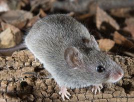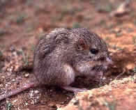
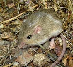
	Baiomys taylori	northern pygmy mouse	Yes, apparently southeastern Arizona counts as 'northern' for this genus. One of two competitors for title of 'smallest Portal rodent,' B. taylori is currently an infrequent but welcome visitor to the site. As it is primarily a grassland species, individuals caught on the site rarely stay for long. Interestingly, the roughly 8-gram B. taylori is often found in association with cotton rats (Sigmodon), which can weight in excess of 100 grams.
	Chaetodipus baileyi	Bailey's pocket mouse	Bailey's pocket mouse made its first appearance on the site in the mid-1990s. It is essentially a giant version of its congeneric relative, the desert pocket mouse (C. penicillatus). While close in size to Merriam's and Ord's kangaroo rats, it is an inferior competitor and, therefore, is found almost solely on kangaroo rat exclosure plots.
	Chaetodipus hispidus	hispid pocket mouse	The hispid pocket mouse looks like a cactus mouse in pocket mouse form; it's the size of C. baileyi with a beautiful lateral orange stripe. C. hispidus has historically been the least frequently recorded species at the site. In the past few months, however, we've caught one or two each trapping period. Nevertheless, it remains a very transient speices; each individual caught this year has been caught once and then never seen again.
	Chaetodipus intermedius	rock pocket mouse	C. intermedius is another pocket mouse, though very rarely found at the site as it prefers rockier habitats; it is very similar to C. penicillatus except in habitat preference.
	Chaetodipus penicillatus	desert pocket mouse	Although C. penicillatus had been found at the site since the beginning of the study, it didn't become such an important player in the system until the 2000s. Now, this small pocket mouse is one of the main seasonal drivers of total rodent abundance at the site. The population explodes in the summers with known individuals, new adults, and brand new babies alike; they are ubiquitous across the site, regardless of plot type. In the winters, C. penicillatus enters a type of torpor (not quite hibernation), creating a large seasonal fluctuation in abundance.
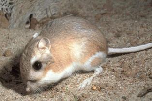
	Dipodomys merriami	Merriam's kangaroo rat	Kangaroo rats, with their giant hind feet and namesake bipedal movement, are some of the most beloved species at the site. Of the three species in the Dipodomys genus, D. merriami is currently the most abundant and, presumably, dominant in the system.
	Dipodomys ordii	Ord's kangaroo rat	Ord's kangaroo rat is nearly indistinguishable from Merriam's kangaroo rat except for a tiny fifth toe on its hind feet that the Merriams lack. D. ordii can be thought of as D. merriami's kid brother who's always aspiring to be like his brother but can't quite keep up; a grass-loving species, D. ordii is often just trailing D. merriami in abundance.
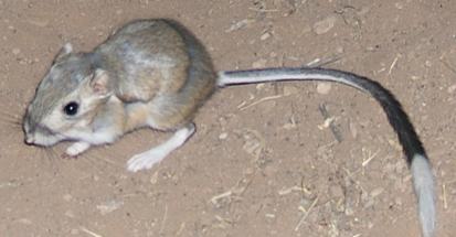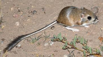
	Dipodomys spectabilis	banner-tailed kangaroo rat	The largest of the three kangaroo rats at the site, D. spectabilis (fondly referred to as 'spectabs' by those in the know) is known for its striking tail. It has by far the largest feet on the site at a whopping 48 mm average and often weighs in at over 100 grams, nearly twice the size of the other kangaroo rats. Spectabs were once running the show at Portal. As the site became shrubbier, however, the reign of D. spectabilis came to a slow end in the 1990's. Since then, a few individuals have popped up here and there but haven't stuck around, often heading for grassier pastures.
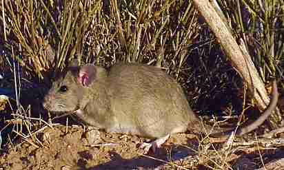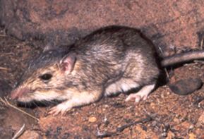
	Neotoma albigula	white-throated woodrat	Along with being by far the largest rodent species at the site (my, what big teeth you have...), Neotoma albigula also has a big reputation---roughly 200 grams worth. Woodrats are quite different ecologically from the rest of the species at the site. Unlike the majority of our rodents which are granivorous, N. albigula is primarily a foliovore. (The resident woodrat in our ramada, however, seems to eat just about anything.) Woodrats---also commonly known as packrats---build middens, or large nests, out of sticks and any 'interesting' debris they can get their paws on. While their numbers at the site aren't prolific, research assistants know exactly which kangaroo rat exclosure plots this species tends to inhabit and secretly wish they'd brought leather gloves with them.
	Onychomys leucogaster	northern grasshopper/scorpion mouse	Amongst smammal enthusiasts such as ourselves, the carnivorous grasshopper mice (Onychomys genus) are legendary. Their name(s) and [this video](https://www.youtube.com/watch?v=ohd_mSIWTXk) basically say it all. In addition to eating insects and scorpions, they have been known to eat venomous centipedes and even other mice. Both species also have a distinctive high-pitched 'howl' when defending their territory. Mighty though they are, both species, and O. leucogaster in particular, have hilariously short tails. For unknown reasons, the northern grasshopper mouse is less common at the site than the southern.
	Onychomys torridus	southern grasshopper/scorpion mouse	Aside from overall range, the southern species differs little from the northern (O. leucogaster) except for a slightly longer tail and somewhat more elongated appearance. This species is more abundant at the site and can be found in all plot types.
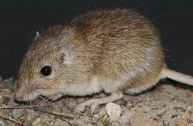
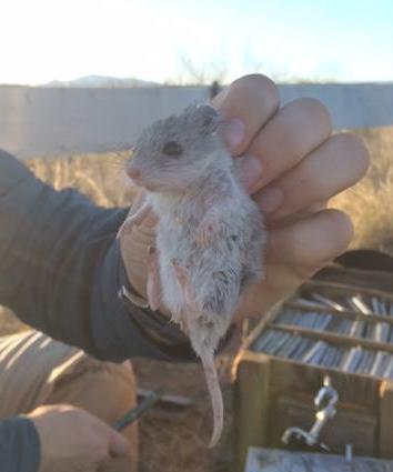
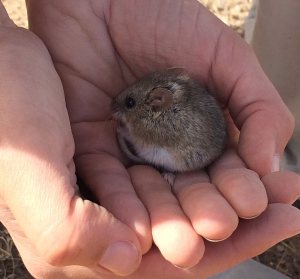
	Perognathus flavus	silky pocket mouse	Perognathus flavus rivals only Baiomys taylorii for the title of smallest rodent at our site, weighing between 5 and 10 grams. Tiny, beautiful, and immensely soft, this aptly named silky pocket mouse is a favorite of previous and current research assistants alike. Its relatively low abundance and recent rarity makes it an especially exciting catch.
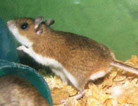
	Peromyscus eremicus	cactus mouse	Often having a bold lateral orange stripe, the cactus mouse is one of the most colorful and striking mice at Portal. It is also the most commonly found Peromyscus species at the site, usually found in kangaroo rat exclosures and incidentally in the full removal plots. Unlike the white-footed mouse and deer mouse, however, it is mainly restricted to the deserts in the American Southwest and northern Mexico.
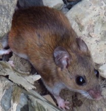	Peromyscus leucopus	white-footed mouse	This Peromyscus species, while very common throughout the majority of the United States, is not all that common at Portal. Peromyscus are good climbers and, therefore, frequently end up in the full rodent exclosure plots.
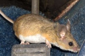
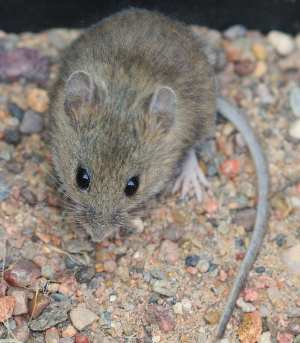
	Peromyscus maniculatus	deer mouse	Like P. leucopus, P. maniculatus is nearly ubiquitous throughout the continental United States but is not a particularly common resident at the site. The desert variants of these two species are challenging to distinguish between, adding a fun challenge to trapping.
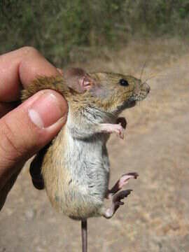	Reithrodontomys fulvescens	fulvous harvest mouse	The fulvous harvest mouse is an infrequent visitor to the site. It is the largest---and the rarest---harvest mouse species found at the site. Like many of the Reithrodontomys caught at the site, it is most often found in kangaroo rat exclosures and full rodent removals.
	Reithrodontomys megalotis	western harvest mouse	R. megalotis is the most common harvest mouse found at Portal. Harvest mice abundance tends to remain fairly low throughout the site, though there is sometimes an increase in the winter when the desert pocket mice (C. penicillatus) are in torpor.
	Reithrodontomys montanus	plains harvest mouse	While very similar to R. megalotis, R. montanus is notably smaller than the other harvest mice at the site. It is less commonly found at the site than R. megalotis but plays a similar role ecologically.
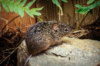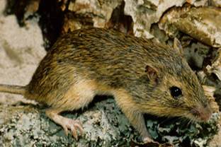
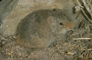
	Sigmodon fulviventer	tawny-bellied cotton rat	A favorite of many Portal research assistants, rodents in the Sigmodon genus are best described as 'squishy like cotton.' Okay, so maybe that's not the most descriptive identifier, but their size and coloration make them an easily identifiable genus. S. fulviventer is one of the two more frequently seen cotton rat species at the site. It is distinguishable by the yellow (rather than white) fur on its belly, as indicated by its descriptive common name.
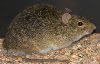	Sigmodon hispidus	white-bellied cotton rat	S. hispidus, with a white rather than a tawny belly, is the other cotton rat species that somewhat frequently has been caught at the site. The Sigmodons seem to come through the site in waves; some years are boom years while others are bust years. What is driving these population cycles? How do Sigmodons move through the regional landscape? We don't know but sure would like to find out.
	Sigmodon ochorognathus	yellow-nosed cotton rat	S. ochorognathus almost seems like an urban (erm...rural) legend nowadays. A few individuals were caught in the 1990s, but none have been seen since.

These are the covariates (without lags imposed) used in forecasting models. Solid lines are historic data, dashed lines are forecasts.